CIS 5800 · Machine Perception · University of Pennsylvania
Geometric Vision: Homographies to Bundle Adjustment
Recovering scene geometry from images with progressively less given — a planar homography with correspondences supplied, differential flow with none, and finally bundle adjustment solving for camera poses and 3-D structure at once.
Period
Sep – Dec 2025
Stack
Bundle Adjustment · PyTorch · LoFTR · Optical Flow · RANSAC · Homography · OpenCV
Highlights
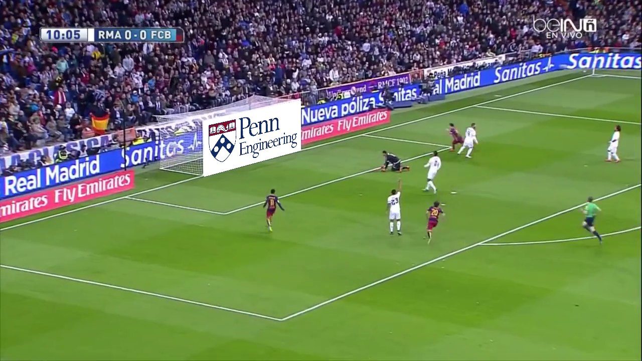
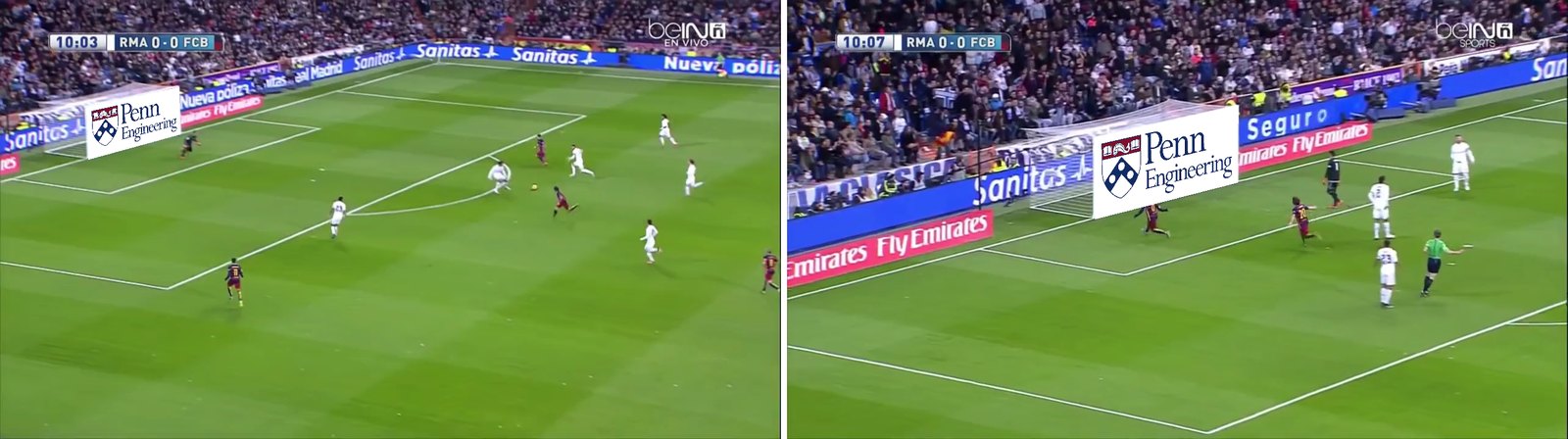
- 01Planar homography by DLT — an 8×9 constraint matrix from four correspondences, solved as the right null vector via SVD, used to composite the Penn Engineering logo into a moving broadcast frame
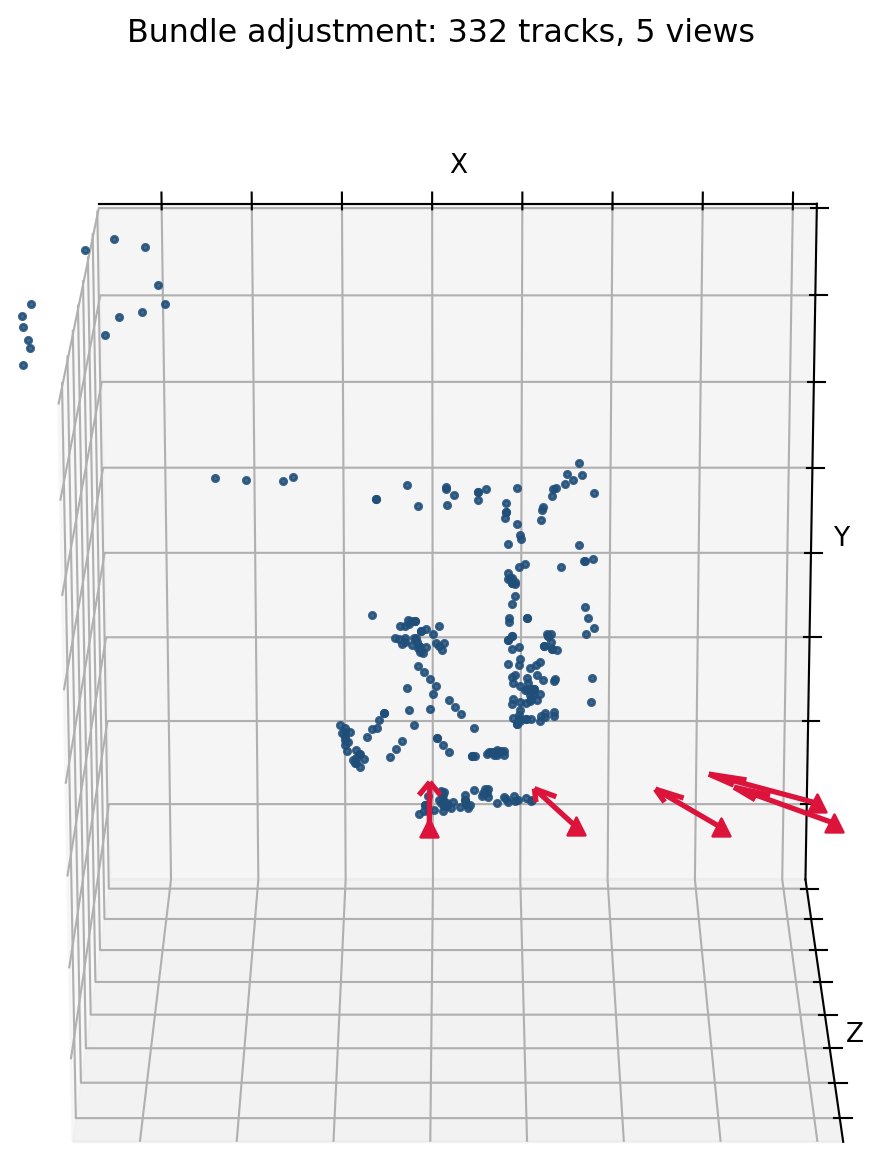
- 02Bundle adjustment written from scratch in PyTorch: axis-angle rotations, translations and N 3-D points as leaf parameters optimised by Adam against a pure reprojection loss, driving the loss from 0.094 to 0.0018
- 03Gauge fixed by holding the first camera at identity — only F−1 poses are parameters, which is what stops the reconstruction from sliding freely in space
- 04LoFTR detector-free matching as an alternative front end: dense pairwise matches filtered at confidence 0.5, then chained across frames by nearest-neighbour association within 3 px to build 330 tracks visible in all five views
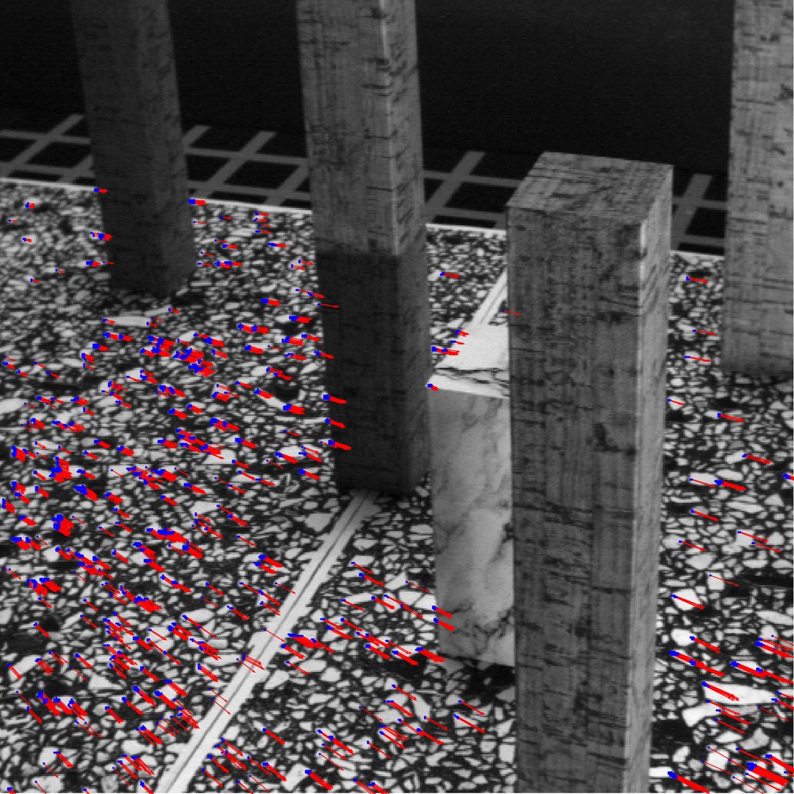
- 05Lucas-Kanade optical flow solved per 5×5 patch by least squares, with the smallest singular value of the patch gradient matrix as a per-pixel confidence score
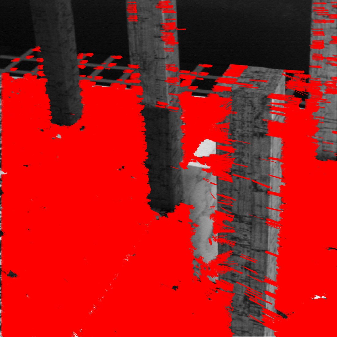
- 06RANSAC recovery of the focus of expansion from flow lines — the confidence threshold cuts 120,212 candidate vectors down to 2,020 before anything is fitted
Results
Write-up
The sequence of problems is really one problem with progressively less handed to you. The homography assumes a plane and is given its correspondences. Optical flow assumes nothing about the scene but has no correspondences at all and has to manufacture them differentially. Bundle adjustment gives up both and solves for camera motion and 3-D structure simultaneously from nothing but tracked points.
The homography itself is four correspondences, an 8×9 constraint matrix and the right null vector from an SVD — short enough that the interesting decision is elsewhere. The warp runs backwards: rather than pushing goal pixels forward into the logo and leaving holes wherever the mapping fails to land on integer coordinates, the interior points of the goal are mapped into logo coordinates and sampled from there. Same H, inverse direction, and the difference between a clean composite and a perforated one.
For bundle adjustment the parameterisation is what makes the optimiser's job possible. Rotations live on SO(3), which a gradient step does not respect; representing each as a three-vector in axis-angle and passing it through Rodrigues makes the parameters unconstrained reals, so Adam can descend on them directly with no orthogonality projection or re-normalisation. The reprojection loss is then just perspective division and a squared difference. Two details decide whether it converges: the first camera is held at identity so the reconstruction has a gauge to be defined against, and the 3-D points initialise at random depth around z = 2 rather than at the origin, because a nonconvex reprojection error started in a degenerate configuration has nowhere useful to go. With both in place the loss falls from 0.094 to 0.0018.
Swapping the front end to LoFTR was less about matching quality than about what bundle adjustment actually needs. LoFTR returns dense pairwise matches with confidences; BA needs tracks — the same physical point identified in every frame. Building those meant matching frame 0 against each later frame separately, then associating the results back through frame 0 by nearest neighbour within a 3 px radius and keeping only the points that survive every association. Each frame added shrinks the surviving set, which is the real cost of insisting on full-length tracks, and the reason the final count lands near the SIFT baseline rather than far above it.
The flow work turns out to be a lesson about confidence rather than about flow. Lucas-Kanade solves a 2×2 least-squares system per patch, and that system is well-conditioned only where the image gradient points in more than one direction — everywhere else the aperture problem means the answer is confidently wrong. Taking the smallest singular value of the patch gradient matrix as a score and thresholding on it drops 120,212 candidate vectors to 2,020, and only then does fitting a focus of expansion by RANSAC over the flow lines make sense. The visible result is that the estimate is carried entirely by the textured gravel while the smooth columns contribute nothing, which is exactly what should happen.