ESE 650 · University of Pennsylvania
Estimation and Learning in Robotics
One question followed through four implementations — how a robot turns noisy measurement into belief. A 2-D Bayes filter, particle-filter SLAM over KITTI LiDAR, a NeRF trained from COLMAP poses, and PPO walking a dm_control biped.
Period
Feb – May 2026
Stack
Particle Filter · SLAM · KITTI · NeRF · PPO · PyTorch · NumPy
Highlights
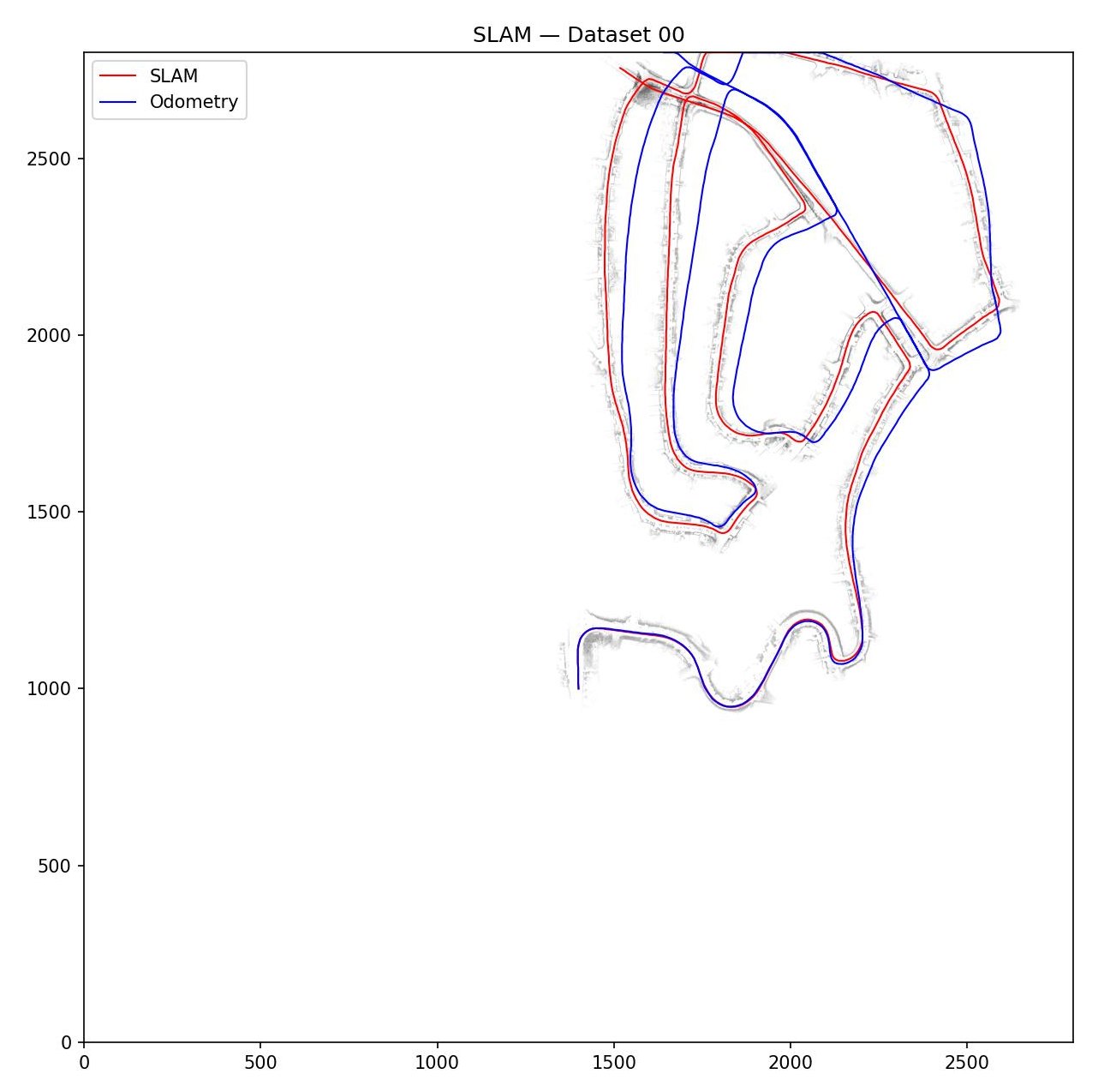
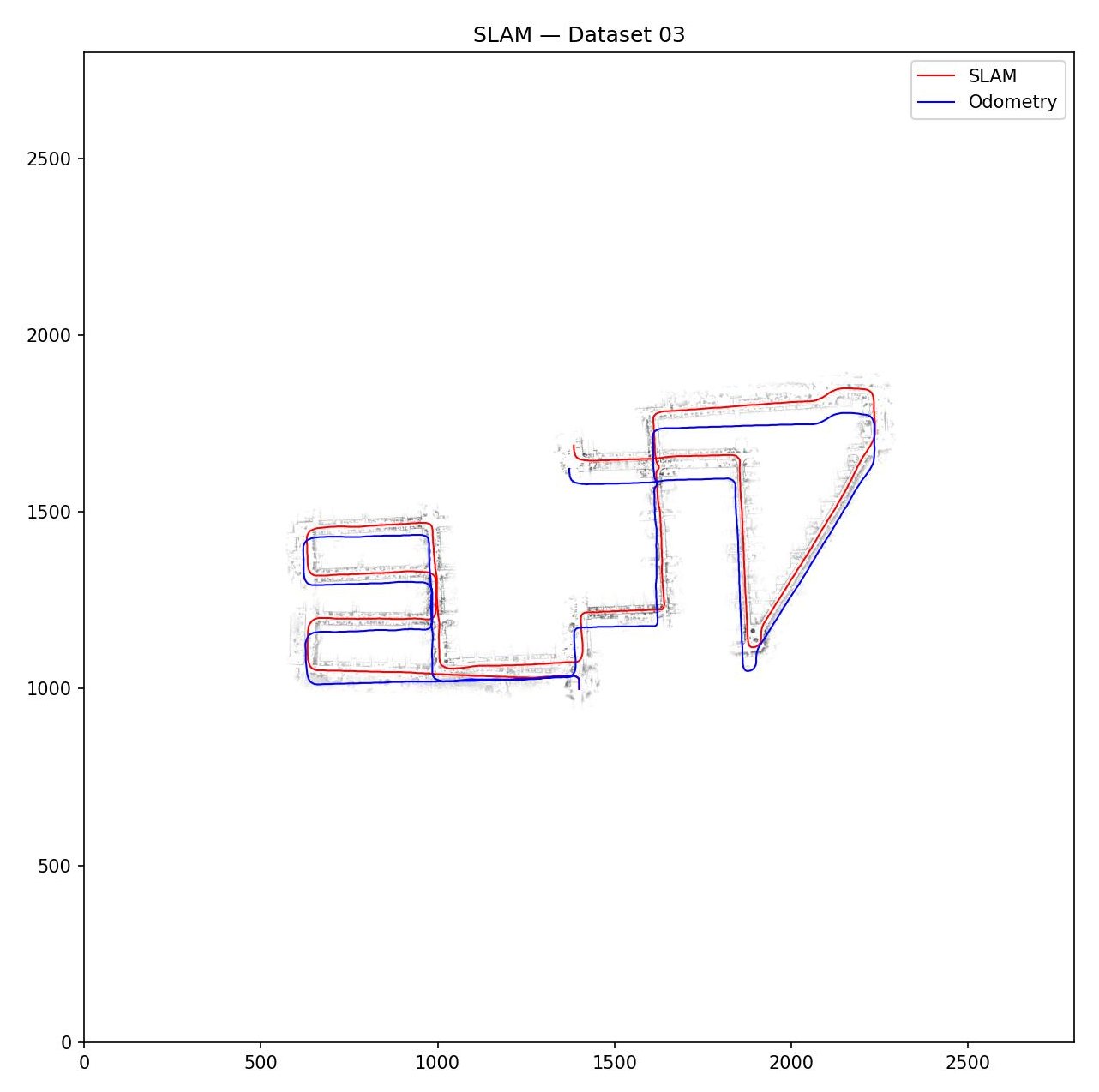
- 01Particle-filter SLAM across four KITTI odometry sequences — log-odds occupancy grid at 0.5 m resolution, Velodyne-to-camera calibration, and stratified resampling triggered when the effective particle count falls below 30%
- 02Scan likelihood scored by correlating the pose-transformed point cloud against the binarised map, with weights normalised in log space by log-sum-exp
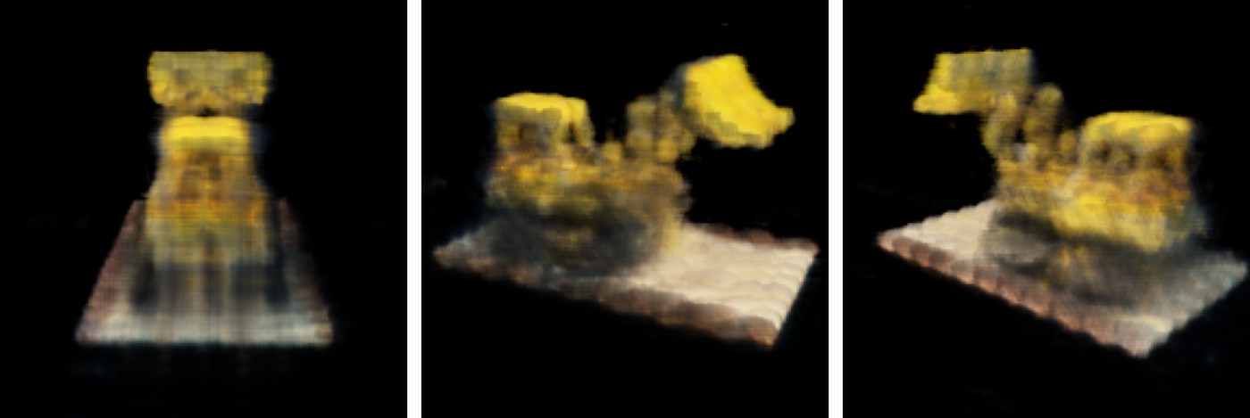
- 03TinyNeRF trained end-to-end on CPU: 63-dimensional positional encoding (L = 10), 32 samples per ray over [2, 6], a three-layer 32-wide MLP, 1000 Adam iterations
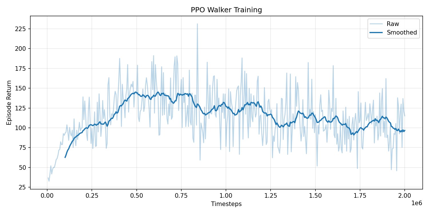
- 04PPO on the dm_control Walker over 2M environment steps — GAE(λ = 0.95), clipped surrogate at 0.2, KL-triggered early stop at 0.05, linear learning-rate decay from 3e-4 to 1e-5
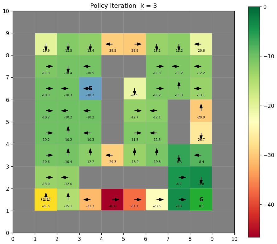
- 05Exact policy iteration on a stochastic 10×10 grid world, solving the Bellman system directly rather than iterating, converged in four improvement sweeps
- 06HMM forward-backward with Baum-Welch re-estimation and a 2-D histogram filter, both written from scratch in NumPy
Results
Write-up
Four assignments that look unrelated on a syllabus — a grid-world filter, LiDAR SLAM, neural rendering, reinforcement learning — are the same question asked with progressively less given: what does the robot believe, and what does a new measurement do to that belief. The belief is a probability grid, then a weighted particle set over pose and map, then a continuous radiance field, then a policy. What changes is the representation; the update is always the same shape.
In the SLAM problem the expensive part is not the map, it is scoring the particles. Each particle transforms the full LiDAR sweep into world coordinates through the Velodyne-to-camera calibration and its own pose hypothesis, and its log-likelihood is the sum of the binarised occupancy map over the cells that sweep lands in — a correlation between what the scan says is there and what the map already believes. Weights update in log space and normalise through log-sum-exp, because doing it in probability space underflows within a few dozen frames. Resampling only fires when the effective particle count drops below 30%, since resampling every step throws away diversity for nothing.
It is worth being precise about what the KITTI plots show, because they are easy to read as more flattering than they are. The control input is the relative motion between consecutive ground-truth poses, perturbed by Gaussian noise. So the filter is not correcting drifting odometry — it is holding an estimate together against noise that was deliberately injected, using a map it is building at the same time. The separation between the red and blue curves is the residual error, and the interesting question is where it grows: in the stretches where the map geometry constrains the pose least.
The NeRF is deliberately small — three hidden layers of width 32, 32 samples per ray, 1000 iterations, trained on CPU at 200×200. At that scale the thing that decides whether anything works at all is the positional encoding. A plain MLP fed raw (x, y, z) is heavily biased toward low frequencies and reconstructs a coloured blur; lifting the input to 63 dimensions with ten octaves of sine and cosine is what lets the same network place an edge. The renders come back with the scene's shape and colour intact and its high-frequency detail gone, and frontal poses reconstruct visibly better than oblique ones, where fewer training rays ever passed through that part of the volume.
The PPO result is the one I would not leave out. Return climbs steadily to about 145 by 500k steps, holds through 800k, then degrades to roughly 95 by the end of the 2M-step budget — this despite a KL-triggered early stop tightened to 0.05 specifically to prevent late-training collapse, and a linearly decaying learning rate. It is a clean demonstration that monotonic improvement is not something PPO gives you, and that training longer is a decision to be justified rather than a free win. The best-return checkpoint is saved separately from the final one, and it is genuinely better than the policy the run ends on.
The grid-world problem closes the loop back to the start. With the transition tensor and reward known, policy evaluation is not an iteration at all — it is a linear solve, exact in one step — and policy iteration converges in four sweeps because each greedy improvement is made over an exactly-evaluated value function. Everything later in the semester is that same computation done approximately, because the model is no longer available.